🧬
🔬 005. Biomedical Segmentation with U-Net
TL;DR
- Build and train a U-Net model for pixel-wise segmentation of microscopy images.
- Covering data preprocessing, augmentation, network architecture, training loop, and evaluation metrics.
In biomedical imaging, accurate delineation of structures—like cell membranes or lesions—is critical. In this post, we'll explore how to implement a U-Net architecture from scratch in Python, train it on a microscopy dataset, and evaluate its performance on unseen samples. You'll see every step: loading images, augmenting data on the fly, defining the encoder-decoder network, and monitoring Dice and IoU metrics.
1. Project Pipeline Overview
- Data Loading: Read raw microscopy images and corresponding binary masks.
- Preprocessing & Augmentation: Resize to 256×256, normalize intensities, and apply flips/rotations.
- Model Architecture: U-Net with contracting and expanding paths, skip connections.
- Training Loop: Batch-wise training with Adam optimizer, monitoring loss and Dice score.
- Evaluation: Compute Intersection-over-Union (IoU) and visualize predicted masks.
2. Data Preparation & Augmentation
We use tf.data to build an efficient pipeline. Images are loaded as 8-bit PNGs, resized, and normalized to [0,1]. Then we apply random flips and rotations.
import tensorflow as tf

AUTOTUNE = tf.data.AUTOTUNE

def load_image(path_img, path_mask):
    img = tf.io.read_file(path_img)
    img = tf.image.decode_png(img, channels=1)
    img = tf.image.resize(img, (256,256)) / 255.0

    mask = tf.io.read_file(path_mask)
    mask = tf.image.decode_png(mask, channels=1)
    mask = tf.image.resize(mask, (256,256)) / 255.0
    mask = tf.round(mask)  # ensure binary

    return img, mask

def augment(img, mask):
    if tf.random.uniform([]) > 0.5:
        img = tf.image.flip_left_right(img)
        mask = tf.image.flip_left_right(mask)
    if tf.random.uniform([]) > 0.5:
        img = tf.image.rot90(img)
        mask = tf.image.rot90(mask)
    return img, mask

def get_dataset(image_paths, mask_paths, batch_size=8):
    ds = tf.data.Dataset.from_tensor_slices((image_paths, mask_paths))
    ds = ds.map(load_image, num_parallel_calls=AUTOTUNE)
    ds = ds.map(augment, num_parallel_calls=AUTOTUNE)
    ds = ds.shuffle(100).batch(batch_size).prefetch(AUTOTUNE)
    return ds
3. U-Net Architecture
U-Net consists of a contracting path (encoder) that captures context and an expanding path (decoder) that enables precise localization through skip-connections.
from tensorflow.keras import layers, Model

def unet_block(inputs, filters):
    x = layers.Conv2D(filters, 3, padding='same', activation='relu')(inputs)
    x = layers.Conv2D(filters, 3, padding='same', activation='relu')(x)
    return x

def build_unet():
    inputs = layers.Input((256,256,1))
    # Encoder
    c1 = unet_block(inputs, 64)
    p1 = layers.MaxPool2D()(c1)
    c2 = unet_block(p1, 128)
    p2 = layers.MaxPool2D()(c2)
    # Bottleneck
    c5 = unet_block(p2, 256)
    # Decoder
    u6 = layers.Conv2DTranspose(128, 2, strides=2, padding='same')(c5)
    u6 = layers.concatenate([u6, c2])
    c6 = unet_block(u6, 128)
    u7 = layers.Conv2DTranspose(64, 2, strides=2, padding='same')(c6)
    u7 = layers.concatenate([u7, c1])
    c7 = unet_block(u7, 64)
    outputs = layers.Conv2D(1, 1, activation='sigmoid')(c7)
    return Model(inputs, outputs)

model = build_unet()
model.compile(optimizer='adam', loss='binary_crossentropy',
              metrics=[tf.keras.metrics.MeanIoU(num_classes=2)])
4. Training & Monitoring
We train for 30 epochs with callbacks to save the best model and reduce learning rate on plateau.
callbacks = [
    tf.keras.callbacks.ModelCheckpoint("unet_best.h5", save_best_only=True),
    tf.keras.callbacks.ReduceLROnPlateau(patience=5, factor=0.5)
]

history = model.fit(
    train_ds,
    validation_data=val_ds,
    epochs=30,
    callbacks=callbacks
)
We visualize loss and IoU curves to verify convergence and generalization.
5. Results & Visualization
Below is a sample input image and our U-Net’s prediction between a possibility map.
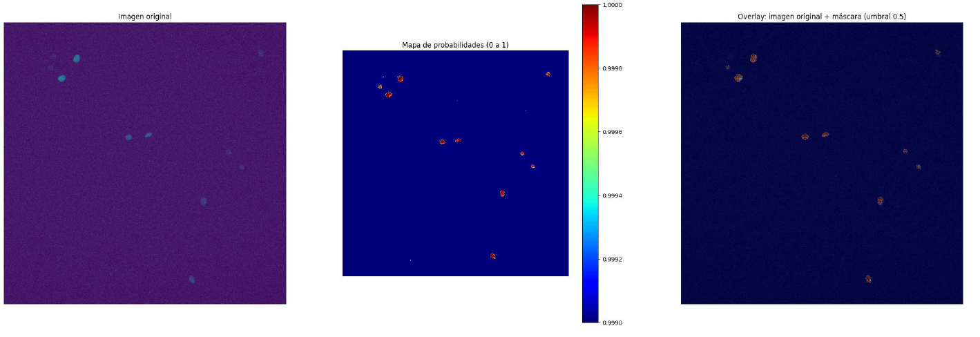
Input Image
6. Conclusion
U-Net remains a gold standard for biomedical segmentation due to its simplicity and effectiveness. With proper preprocessing, augmentation, and diligent monitoring of IoU, you can achieve pixel-level accuracy even on small datasets. Feel free to download the full code and pretrained weights below and adapt it to your own microscopy projects!